pyAPP6 Examples
Content: These examples are grouped into three main sections:
Version: pyAPP6 version 1.0
Note: This example was written as a jupyter notebook (version 4.1.0), and has been tested with Python 2.7.11 |Anaconda 4.0.0 (64-bit). The notebook file is available in the Examples directory of the pyAPP6 distribution.
Imports & Constants
Imports for plotting (matplotlib) and arrays (numpy):
import matplotlib.pyplot as plt
import numpy as np
Jupyter Notebook specific imports:
%matplotlib inline
Constants:
APP6DIR = r'C:\Program Files (x86)\ALR Aerospace\APP 6 Professional Edition'
Files
The Files module is used to open, change and save APP Files. It can be used for: * acft (Aircraft) * mis (Mission Computation) * perf (Performance Charts)
file types.
It is recommended to create a new file using the APP GUI and subsequenty modify this file using Python/pyAPP6, instead of creating a file from scratch with pyAPP6.
Import the pyAPP6 modules
from pyAPP6 import Files
from pyAPP6 import Database
from pyAPP6 import Units
The Units and Database modules are imported as well for this example. They are useful to convert units and translate APP indices to human-readable text
Aircraft File (*.acft)
To load an APP aircraft model, the class AircraftModel is used. A new instance can be created directly with the fromFile class method:
aircraftpath = r'data\\LWF.acft'
acft = Files.AircraftModel.fromFile(aircraftpath)
Now we have the aircraft file available in the acft variable. All data within the aircraft can be accessed through class member variables directly, or by using get functions. This examples shows how to access fields in the General Data tab of APP’s aircraft model GUI:
data = acft.getGeneralData()
print ('Aircraft Name:', data.m_sAircraftName)
print ('Author:', data.m_sAuthor)
('Aircraft Name:', 'LWF')
('Author:', 'ALR')
Getter functions exist for all the main datasets. To print lists of the available data sets, use:
print(acft.getMassLimitsNames())
print(acft.getAeroNames())
print(acft.getPropulsionNames())
print(acft.getStoreNames())
['Standard']
['Cruise', 'TO Flaps 27xb0']
['LWF']
['AIM-9 Wingtip']
This example demonstrates how to loop through an X2Table (in this case the CL/CDi table) and correctly lable the drag polars:
i = 0
aero = acft.getAero(i) #get the first aerodanymic dataset, in this case 'Cruise'

fig = plt.figure(figsize=(8.3, 5.8)) #A5 landscape figure, size is in inches
ax = plt.subplot(1,1,1)

for val, table in zip(aero.cdITable.value,aero.cdITable.table):
    ax.plot(table[:,1], table[:,0], 'd-', label='Mach = '+str(val))

# adjust Axis properties
ax.set_title(acft.getAeroName(i))
ax.legend(loc='best')
ax.set_xlabel('$CD_i$')
ax.set_ylabel('$CL$')
ax.grid()
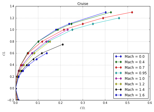
For an detailed explaination of the XTables classes, consult the pyAPP6 user guide.
A more involved example would be to compare lift curves of all available aero datasets:
fig = plt.figure(figsize=(8.3, 5.8)) #A5 landscape figure, size is in inches
ax = plt.subplot(1, 1, 1)
for aero, aeroName in zip(acft.getAeroList(), acft.getAeroNames()):
    ax.plot(aero.clTable.table[0][:,0]*Units._DEG, aero.clTable.table[0][:,1], label=aeroName.decode('cp1252'))

ax.set_xlabel(u'$AoA$ [°]')
ax.set_ylabel(u'$CL$')
leg = ax.legend(loc=2)
#fig.savefig('CL_comparison.png',dpi=200)
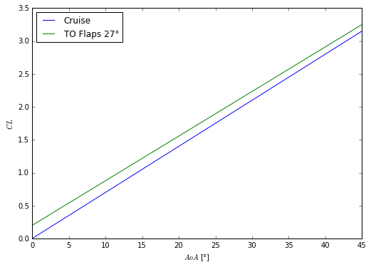
Additionally, this example demonstrates the use of the Units module to convert from radians to degrees.
Note: In oder for the legend label for the TO Flaps 27° setting to be printed correctly, the aeroName string has to be converted to unicode with the enconding of the original text file, in this case cp1252. In addition, to print the ° sign in the x-axis label, the string has to be unicode and is typed with the prefix ‘u’
Mission File (*.mis)
The mission file is loaded using the classmethod fromFile in the MissionComputationFile class:
missionpath = r'data\\LWF Air Combat Mission RoA.mis'
missionFile = Files.MissionComputationFile.fromFile(missionpath)
The file can now be examined and changed via Python. For example, getInitialCondition() can be used to access the initial conditions. The following code changes the initial fuel mass to 80% and the altitude to 1000 m:
initFd = missionFile.getInitialCondition()
initFd.fuel.xx = 0.8
initFd.alt.xx = 1000.0
To loop through the segments, use getSegmentList() to access the list of segments. The following code prints the segment index (identifier) of each segment:
for segment in missionFile.getSegmentList():
    print(segment.segmentIndex)
SEG_GROUNDOP
SEG_TAKEOFF
SEG_CLIMB
SEG_BESTCLIMBRATE
SEG_ACCELERATION
SEG_TARGETMACHCRUISE
SEG_MANEUVRE
SEG_STOREDROP
SEG_MANEUVRE
SEG_STOREDROP
SEG_LOITER
SEG_SPECIFICRANGE
SEG_DECELERATION
SEG_CASDESCENT
SEG_LANDINGROLL
In order to display the label of each segment instead of the index string, you can use the Database class:
db = Database.Database()
for segment in missionFile.getSegmentList():
    print(db.GetTextFromID(segment.segmentIndex))
Ground Operation
Takeoff
Climb
Climb at Best Rate
Acceleration
Cruise at Mach
Maneuver at Max. LF
Store Drop
Maneuver at Max. LF
Store Drop
Loiter
Cruise at Best SR
Deceleration
Descent at CAS
Landing Roll
Similarly, the type and value of the segment end condition can shown:
for segment in missionFile.getSegmentList():
    print(db.GetTextFromID(segment.endValue1.realIdx),':', segment.endValue1.xx, )
('Seg. Time', ':', 600.0)
('Velocity', ':', 75.4455900943)
('Altitude', ':', 500.0)
('Altitude', ':', 9500.0)
('Mach', ':', 0.9)
('Seg. Dist.', ':', 320053.202172)
('Turns', ':', 12.5663706144)
('Seg. Time', ':', 100.0)
('Turns', ':', 6.28318530718)
('Seg. Dist.', ':', 100.0)
('Seg. Time', ':', 600.0)
('Seg. Dist.', ':', 402135.694779)
('CAS', ':', 102.888888976)
('Altitude', ':', 500.0)
('Velocity', ':', 0.01)
In order to change the altitude of the segment “Climb at Best Rate” (Segment index 3) from 9500m to 7000m, do:
print(missionFile.getSegment(3).endValue1.xx)
missionFile.getSegment(3).endValue1.xx = 7000.0
print(missionFile.getSegment(3).endValue1.xx)
9500.0
7000.0
Also change the altitude of the initial climb after takeoff (Segment index 2) to 500m above the starting altitude.
print(missionFile.getSegment(2).endValue1.xx)
missionFile.getSegment(2).endValue1.xx = initFd.alt.xx + 500.0
print(missionFile.getSegment(2).endValue1.xx)
500.0
1500.0
missionpath_mod = r'data\\LWF Air Combat Mission RoA_mod.mis'
missionFile.saveToFile(missionpath_mod,overwrite=True)
Performance Chart File (*.perf)
A PerformanceChartFile is instantiated via the fromFile classmethod:
chartpath = r'data\\LWF Climb Rate Chart 50% Fuel.perf'
chart = Files.PerformanceChartFile.fromFile(chartpath)
This example shows how to change the flight state (initial condition). The function getInitialCondition returns an instance of type FlightData:
fd = chart.getInitialCondition()
print fd.alt.xx
print fd.speed.xx, db.GetTextFromID(fd.speed.realIdx) #Mach Number
print fd.fuel.xx, db.GetTextFromID(fd.fuel.realIdx)
0.0
0.0 Mach
0.5 Fuel Percent
Note: the speed variable can be either Mach or TAS. Check the corresponding realIdx string. Similarly, the variables payload, climb, thrust and pull can be of different type
Change the fuel from the current state (50%) to 100%
print(fd.fuel.xx)
0.5
fd.fuel.xx = 1.0
To change the aircraft Configuration, for example from Dry (configuration index 0) to Reheat (configuration index 1), access the ProjectAircraftSetting class. To see what configurations are available, open the aircraft model.
configNames = acft.getConfigurationNames()
print 'Configurations in the aircraft model:\n', configNames, '\n'

cfg = chart.getAircraftConfiguration()
print cfg.activeSetting, configNames[cfg.activeSetting]
cfg.activeSetting = 1
print cfg.activeSetting, configNames[cfg.activeSetting]
Configurations in the aircraft model:
['Cruise, Dry', 'Cruise, Reheat', 'TOL, Reheat', 'TOL, Dry']

0 Cruise, Dry
1 Cruise, Reheat
Similarly, External Store Configurations can be changed:
storeConfigNames = acft.getStoreConfigurationNames()
print 'Store configurations in the aircraft model:\n',storeConfigNames,'\n'

cfg = chart.getAircraftConfiguration()
print cfg.activeStoreSetting, storeConfigNames[cfg.activeStoreSetting]
cfg.activeStoreSetting = -1 #use -1 for no external stores (clean)
Store configurations in the aircraft model:
['Air-to-Air']

0 Air-to-Air
To access the computation, use the getComputation method. The type of performance chart can be checked with the CompType variable. In the case of a Point Performance Computation, the type of equation solved is stored in resData.CmpType.
comp = chart.getComputation()
print db.GetTextFromID(comp.CompType)
print db.GetTextFromID(comp.resData.CmpType)
Point Performance Computation
Climb
The resData attribute also holds the data ranges for the chart in two X0Tables, one for the X-Range the other for the Parameter:
print comp.resData.X1Range.X0Typ
print comp.resData.X1Range.table

print comp.resData.X2Range.X0Typ
print comp.resData.X2Range.table
REAL_MACH
[ 0.2   0.25  0.3   0.35  0.4   0.45  0.5   0.55  0.6   0.65  0.7   0.75
  0.8   0.85  0.9   0.95]
REAL_ALT
[     0.   2500.   5000.   7500.  10000.]
For example, to change the computed altitudes, replace the table with a new numpy array:
comp.resData.X2Range.table = np.linspace(0.0, 10000.0, 3)
print comp.resData.X2Range.table
[ 0. 5000. 10000.]
or, add values manually (as floats):
comp.resData.X2Range.table = np.array([0.0, 10000.0])
print comp.resData.X2Range.table
[ 0. 10000.]
Save your modified file:
chartpath_mod = r'data\\LWF Climb Rate Chart 100% Fuel.perf'
chart.saveToFile(chartpath_mod, overwrite=True)
Mission Computation
Import the Mission module from pyAPP6:
from pyAPP6 import Mission
In order to run APP mission computations, create an instance of the MissionComputation class. The path to the directory where the APP executable can be found has to be provided
misCmp = Mission.MissionComputation(APP6Directory = APP6DIR)
misCmp.run(missionpath)
True
res = misCmp.result
Access data by looping through the segments. To get a specific variable, find the index of the variable by using the function getVariableIndex. To access the data of the segment, use getData. getData returns a 3d numpy array, with the first dimension being the datapoint and the second dimension the variable. For example, the variable Fuel Mass at the end of each segment can be obtained by using:
idx_fuel = res.getVariableIndex('Fuel Mass')

for seg in res.getSegmentList():
    print res.getVariableName(idx_fuel),':',seg.getData()[-1,idx_fuel]
Fuel Mass [kg] : 1896.22
Fuel Mass [kg] : 1859.49
Fuel Mass [kg] : 1779.27
Fuel Mass [kg] : 1532.93
Fuel Mass [kg] : 1520.89
Fuel Mass [kg] : 1123.86
Fuel Mass [kg] : 914.584
Fuel Mass [kg] : 914.584
Fuel Mass [kg] : 815.506
Fuel Mass [kg] : 815.506
Fuel Mass [kg] : 619.614
Fuel Mass [kg] : 225.152
Fuel Mass [kg] : 222.696
Fuel Mass [kg] : 104.648
Fuel Mass [kg] : 100.12
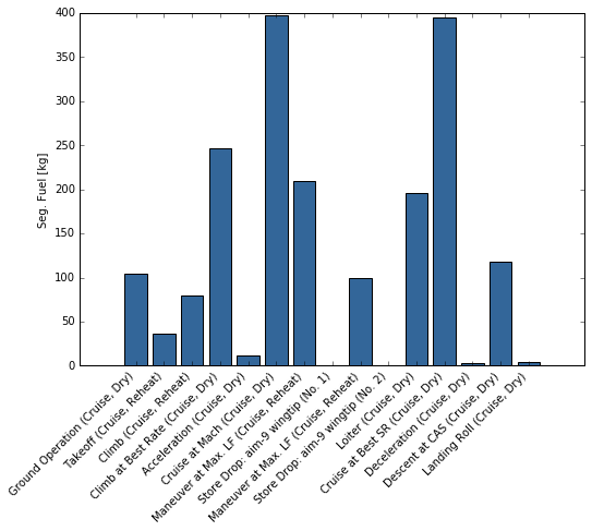
A list of the fuel consumed per segment can be easily ontained using a list comprehension:
idx_segFuel = res.getVariableIndex('Seg. Fuel')

segFuelList = [seg.getData()[-1,idx_segFuel] for seg in res.getSegmentList()]
print segFuelList
[103.782, 36.7258, 80.217600000000004, 246.34299999999999, 12.043900000000001, 397.024, 209.279, 0.0, 99.078299999999999, 0.0, 195.892, 394.46100000000001, 2.4563700000000002, 118.047, 4.5279800000000003]
fig = plt.figure(figsize=(8.3, 5.8)) #A5 landscape figure, size is in inches
ax = plt.subplot(1,1,1)
ax.bar(range(len(segFuelList)),
       segFuelList,
       align='center',
       color='#336699')
ax.set_xticks(range(len(segFuelList)))
ax.set_xticklabels(res.getSegmentNameList(), rotation=45, ha='right')
ax.set_ylabel(res.getVariableName(idx_segFuel))
<matplotlib.text.Text at 0x8454ef0>
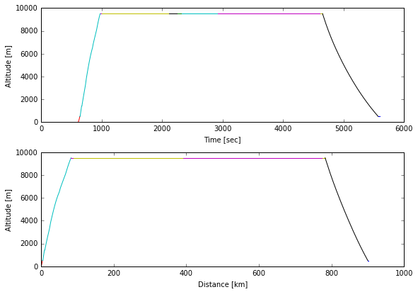
Looping through the segments can also be useful to plot the mission profile:
idx1 = res.getVariableIndex('Time')
idx2 = res.getVariableIndex('Distance')
idx3 = res.getVariableIndex('Altitude')
fig = plt.figure(figsize=(8.3, 5.8)) #A5 landscape figure, size is in inches

ax = plt.subplot(2,1,1)
for seg in res.getSegmentList():
    ax.plot(seg.getData()[:,idx1],seg.getData()[:,idx3])

ax.set_xlabel(res.getVariableName(idx1))
ax.set_ylabel(res.getVariableName(idx3))

ax = plt.subplot(2,1,2)
for seg in res.getSegmentList():
    ax.plot(seg.getData()[:,idx2],seg.getData()[:,idx3])

ax.set_xlabel(res.getVariableName(idx2))
ax.set_ylabel(res.getVariableName(idx3))

plt.tight_layout()
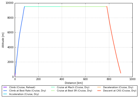
Matplotlib offers a lot of formatting options for legends: http://matplotlib.org/api/legend_api.html#matplotlib.legend.Legend
idx1 = res.getVariableIndex('Distance')
idx2 = res.getVariableIndex('Altitude')
idx_segDst = res.getVariableIndex('Seg. Dist')

fig = plt.figure(figsize=(8.3, 5.8)) #A5 landscape figure, size is in inches
ax = plt.subplot(1,1,1)

colormap = plt.cm.rainbow
ax.set_prop_cycle('color',[colormap(i) for i in np.linspace(0, 0.9, 7)])

for i,seg in enumerate(res.getSegmentList()):
    if seg.getData()[-1,idx_segDst]>2.0:
        ax.plot(seg.getData()[:,idx1], seg.getData()[:,idx2], label=seg.getName(),lw=2.0)

ax.set_xlabel(res.getVariableName(idx1))
ax.set_ylabel(res.getVariableName(idx2))
plt.subplots_adjust(bottom=0.2)
ax.legend(bbox_to_anchor=(1.05,-0.1), ncol=3, fontsize = 9, handlelength = 2.0)
ax.grid()
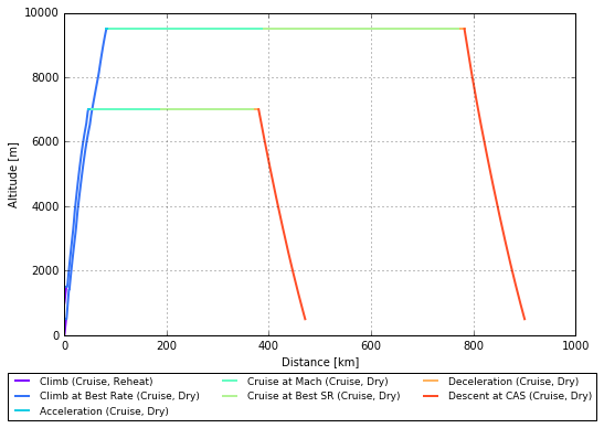
misCmp_mod = Mission.MissionComputation(APP6Directory = APP6DIR)
misCmp_mod.run(missionpath_mod)
True
res_mod = misCmp_mod.result
idx_segDst = res.getVariableIndex('Seg. Dist')
fig = plt.figure(figsize=(8.3, 5.8)) #A5 landscape figure, size is in inches
ax = plt.subplot(1,1,1)

colormap = plt.cm.rainbow
ax.set_prop_cycle('color',[colormap(i) for i in np.linspace(0, 0.9, 7)])

for i,seg in enumerate(res.getSegmentList()):
    if seg.getData()[-1,idx_segDst]>2.0:
        ax.plot(seg.getData()[:,idx1], seg.getData()[:,idx2], label=seg.getName(),lw=2.0)

for i,seg in enumerate(res_mod.getSegmentList()):
    if seg.getData()[-1,idx_segDst]>2.0:
        ax.plot(seg.getData()[:,idx1], seg.getData()[:,idx2],lw=2.0)

ax.set_xlabel(res.getVariableName(idx1))
ax.set_ylabel(res.getVariableName(idx2))
plt.subplots_adjust(bottom=0.2)
ax.legend(bbox_to_anchor=(1.05,-0.1), ncol=3, fontsize = 9, handlelength = 2.0)
ax.grid()
The result of a mission computation can also be loaded from the result text-file after the computation:
resfile = r'data\\LWF Air Combat Mission RoA.mis_output.txt'
res = Mission.MissionResult.fromFile(resfile)
Complex Mission Loop
cap_path = r'data\\LWF CAP Loop.mis'
cap_path_mod = r'data\\LWF CAP Loop_mod.mis'
mis = Files.MissionComputationFile.fromFile(cap_path)
[(i, seg.getName()) for i, seg in enumerate(mis.getSegmentList())]
[(0, 'SEG_GROUNDOP'),
 (1, 'SEG_TAKEOFF'),
 (2, 'SEG_CLIMB'),
 (3, 'SEG_BESTCLIMBRATE'),
 (4, 'SEG_ACCELERATION'),
 (5, 'SEG_TARGETMACHCRUISE'),
 (6, 'SEG_LOITER'),
 (7, 'SEG_STOREDROP'),
 (8, 'SEG_STOREDROP'),
 (9, 'SEG_MANEUVRE'),
 (10, 'SEG_SPECIFICRANGE'),
 (11, 'SEG_NOCREDIT')]
idx_loiter = 6
idx_combat = 9
range_combat = np.linspace(0, 10, 6) # minutes
Read a CAP mission from an existing file, adjust the end-value of the combat segment and save the mission to another file. Afterwards, run the mission, extract the result and store it to a list (i.e. loiter_time).
loiter_time = []
for i in range_combat:
    misFile = Files.MissionComputationFile.fromFile(cap_path)
    combat = misFile.getSegment(idx_combat)
    combat.endValue1.xx = i*60.0 # convert minutes to seconds
    misFile.saveToFile(cap_path_mod, overwrite=True)

    mis = Mission.MissionComputation(APP6DIR)
    mis.run(cap_path_mod)

    res = mis.getResult()

    idx_segTime = res.getVariableIndex('Seg. Time')
    loiter_time.append(res.getSegment(idx_loiter).getData()[-1,idx_segTime])
Plot the results as a bar-chart.
fig = plt.figure(figsize=(8.3, 5.8)) #A5 landscape figure, size is in inches
ax = plt.subplot(1,1,1)
width = 1.4
ax.bar(left=range_combat-2.0*width,
       height=loiter_time, width=width,
       tick_label=[str(c) for c in range_combat],
       align='center',
       color='#336699')
ax.set_title('Combat Air Patrol (CAP)')
ax.set_xlabel('Combat Time [min]')
ax.set_ylabel('Time on Station [min]')
<matplotlib.text.Text at 0x93027f0>
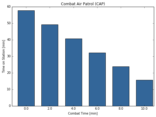
Note: input data is always in SI units (e.g. the combat time segment endValue is in seconds), but the output values are formatted (e.g. loiter time is in minutes)
Performance Charts
Import the Performance module from pyAPP6
from pyAPP6 import Performance
perf = Performance.PerformanceChart(APP6Directory=APP6DIR)
perf.run(chartpath)
True
The result is loaded into a PerformanceChartResult instance:
res = perf.result
A PerformanceChartResult contains a list of ResultLine objects. The ResultLine contains the data as a 2d numpy array, with the first dimension being the datapoints and the second dimension the variable index:
line = res.getLine(0)
data = line.getData()
print data.shape
print data
(16L, 74L)
[[  3.01753000e+04   0.00000000e+00   0.00000000e+00 ...,   6.80588000e+01
    6.49318000e+01   0.00000000e+00]
 [  5.57759000e+04   0.00000000e+00   0.00000000e+00 ...,   8.50735000e+01
    7.92340000e+01   0.00000000e+00]
 [  7.24756000e+04   0.00000000e+00   0.00000000e+00 ...,   1.02088000e+02
    9.46049000e+01   0.00000000e+00]
 ...,
 [  5.32038000e+04   0.00000000e+00   0.00000000e+00 ...,   2.89250000e+02
    2.88040000e+02   0.00000000e+00]
 [  4.42996000e+04   0.00000000e+00   0.00000000e+00 ...,   3.06265000e+02
    3.06247000e+02   0.00000000e+00]
 [  2.83537000e+04   0.00000000e+00   0.00000000e+00 ...,   3.23279000e+02
    3.15662000e+02   0.00000000e+00]]
To find the index of the desired variable, use the getVariableIndex function:
idx1 = res.getVariableIndex('CAS')
idx2 = res.getVariableIndex('Climb Speed')
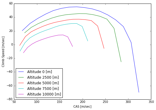
The lines can then be plotted using Matploltib:
fig = plt.figure(figsize=(8.3, 5.8)) #A5 landscape figure, size is in inches
ax = plt.subplot(1,1,1)

#Plot the lines
for line in res.getLineList():
    ax.plot(line.getData()[:,idx1],line.getData()[:,idx2], label=line.getLabel())

ax.legend(loc=3)
ax.set_xlabel(res.getVariableName(idx1))
ax.set_ylabel(res.getVariableName(idx2))
<matplotlib.text.Text at 0x8f8f2b0>
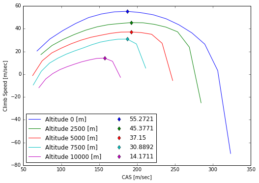
Since each data line is a numpy array, data can easily be processed using the powerful functions of numpy. This example extracts the maxima of each line and plots them. Note: the line contains NaNs, therefore the function np.nanargmax is used to extract the maxima.
fig = plt.figure(figsize=(8.3, 5.8)) #A5 landscape figure, size is in inches
ax = plt.subplot(1,1,1)

#Plot the lines
for line in res.getLineList():
    ax.plot(line.getData()[:,idx1], line.getData()[:,idx2], label=line.getLabel())

ax.set_prop_cycle(None) #Resets the color cycle

#Plot the maxima
for line in res.getLineList():
    xdata = line.getData()[:,idx1]
    ydata = line.getData()[:,idx2]
    idx_max = np.nanargmax(ydata) #find the location of the maximum
    ax.plot(xdata[idx_max], ydata[idx_max], 'd', label=str(ydata[idx_max]))

ax.legend(loc=3, numpoints=1, ncol=2)
ax.set_xlabel(res.getVariableName(idx1))
ax.set_ylabel(res.getVariableName(idx2))
<matplotlib.text.Text at 0x92ec9e8>